Regression Analysis with Python and Numpy

April 20, 2020

Regression analysis is a technique used for finding relationships between dependent and independent variables. Using it, we can better estimate trends in datasets that would otherwise be difficult to deduce.

One method of achieving this is by using Python’s Numpy in conjunction with visualization in Pyplot.

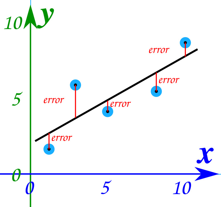
Numpy has a number of functions for the creation and manipulation of polynomials. For this example we will be using the polyfit() function that generates a least squares fitting. Least squares fitting is essentially the reduction of total error in the vertical distance from data points to the fitted function.

For this example, we’ll be plotting a varying dateset comprising the Consumer Price Index for the last 21 years which measures price changes for commonly purchased goods like transportation and food.

# Source data
x_data = [2000,
          2001,
          2002,
          2003,
          2004,
          2005,
          2006,
          2007,
          2008,
          2009,
          2010,
          2011,
          2012,
          2013,
          2014,
          2015,
          2016,
          2017,
          2018,
          2019,
          2020]
y_data = [107.754,
          112.700,
          110.608,
          111.538,
          124.977,
          126.985,
          125.469,
          140.119,
          148.507,
          128.978,
          133.586,
          145.819,
          147.449,
          149.176,
          156.573,
          147.479,
          140.674,
          139.677,
          137.005,
          140.743,
          146.396]
degree = 2

# Generate regression polynomial
polynomial_coefficients = numpy.polyfit(x_data, y_data, degree)

# Format polynomial
formatted_polynomial = numpy.poly1d(polynomial_coefficients)

# Generate data from first and last entry in array
interval = numpy.linspace(x_data[0], x_data[-1])

Our dataset has 21 entries labeled x_data and y_data. We can use this in addition to our requested polynomial degree argument in the polyfit() function. The degree parameter will determine how closely your resulting polynomial tracks your dateset. We’ll see how this value affects the outcome shortly.

# Generate regression polynomial
polynomial_coefficients = numpy.polyfit(x_data, y_data, degree)

This function will only return your polynomial’s coefficients in an array format. In order to use the polynomial like a more standard f(x) function, you can pass your coefficients to poly1d() and use its return value as a function directly!

# Format polynomial
formatted_polynomial = numpy.poly1d(polynomial_coefficients)

Now that you have your fitted polynomial, you’ll need an array of evenly spaced numbers over the interval you’d like to plot. This can be accomplished by taking the first and last entry of your x_data array and passing them into the linspace() function. The amount of values it returns is variable and will return 50 in total by default.

# Generate data from first and last entry in array
interval = numpy.linspace(x_data[0], x_data[-1])

From here it’s simply a matter of handing over your values to Pyplot:

# Configure and display plots
fig, cx = plt.subplots()

# Plot initial dataset
cx.plot(x_data, y_data, '.k')

#Plot fitted polynomial over linspace interval
cx.plot(interval, formatted_polynomial(interval), '-g')

# Enable grid lines
cx.grid()

# Limit default maximum y value to largest polynomial result plus buffer
cx.set_ylim(0, formatted_polynomial(interval).max()*1.5)

plt.show()

The only nonstandard thing I’ve done here is change the set_ylim upper bound to a value a bit higher than the largest number for better view-ability.

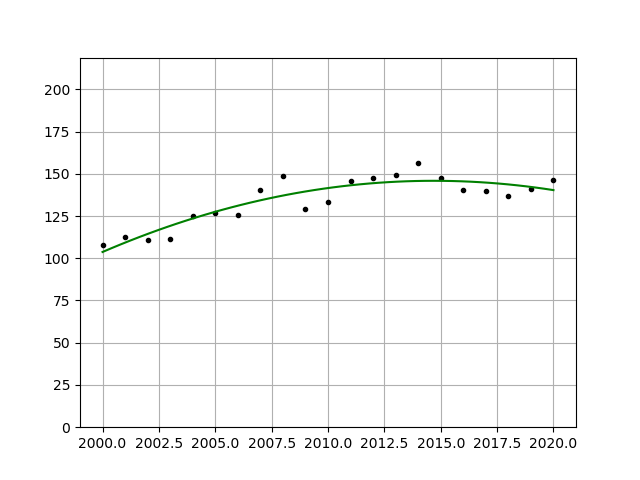
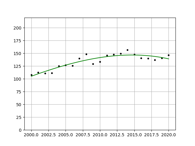
Now this just shows a 2^nd degree polynomial. To more precisely fit your data, you can choose to increase the degree value in your polyfit function. Here is an example of a 3^rd and 4^th degree fitting:

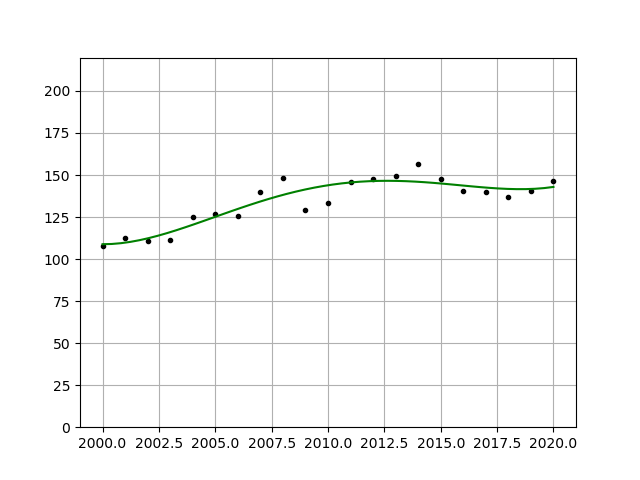
This value can theoretically be increased to a point where your curve fits every single data point perfectly, but this results in over-fitting which is a separate discussion entirely.

Source code can be found here!

Sources

[1] – https://www.mathsisfun.com/data/least-squares-regression.html